Password Protect Excel File

There are two reasons you want to password protect your excel file. Either you do not want other people to see sensitive data in you excel file without your permission or you want to restrict user from modifying your excel file. It can easily be achieved using Microsoft Excel only without using any third party password protection software. In this tutorial I am going to show you how you can password protect your excel file with excel only.

Password Protection Options

Excel files can be password protected using Microsoft excel in two ways.

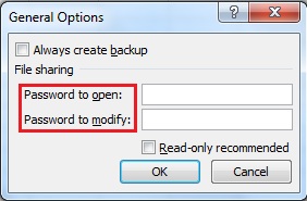
1. Password to Open: When you want to prevent the users from seeing the data in your excel file then use this protection. User will need a password to view the contents of the file.
2. Password to Modify: You want to allow your users to see the data but want to restrict them from making any changes in your excel file, then this is the best option.

How to Password Protect Excel File

Open the file you want to protect and follow these simple steps to password protect you excel files.

1. Go to File menu and click on "Save As". A pop-up window for saving you document will appear on you screen.
2. Click on the "Tools" button on the bottom right hand corner and select "General option..". See image below.
3. Enter a password to protect your document and then click "OK". (See Image below).

Save As

General Options..

Search Box to Search and Display Data

---

In this excel tutorial, we are going to learn how to make a search box. After creating search box, we will use it to search and display data from the database. In the above video you can see what we are going to create in this tutorial. We are going to do this in two steps.

1. Creating search box.
2. Displaying search result.

Creating Search Box 

In this section we are going to create search box and the display box. Instruction for creating search box and display box are given below.

1. Select cells "C2:E2" and click on "Merge & Center".
2. Select all the cell around the merged cells and fill it with black color.
3. Click on "B2". Change font color to white, font size to 12 and make it bold then type "Search".
4. Select cells B5 to F5, hold Ctrl and select C6:F6, C7:F7, C8:F8, C9:F9, C10:F10, C11:F11 and C12:F12 and click on "Merge & Center".
5. Fill with color as shown in the picture above.
6. Click "B5" hold Shift and click on F12.
7. Click on "Thick Box Border" from the border options.

Displaying Search Result 

Here is the sample data which I will be using in this tutorial to show you how you can search and data from the data base.

Click Image to Enlarge

1. Go to Sheet 2 in the same workbook.
2. Click on the formula tab and then "Define Names".
3. Create the following named ranges i.e. Name, Age, Gender, Phone, Email, Address, and Country and type in the following formulas in "Refers to:" text box respectively

• "=OFFSET(Sheet2!$A$2,0,0,COUNTA(Shee2!$A:$A)-1)" 
• "=OFFSET(Sheet2!$B$2,0,0,COUNTA(Shee2!$B:$B)-1)"
• "=OFFSET(Sheet2!$C$2,0,0,COUNTA(Shee2!$C:$C)-1)"
• "=OFFSET(Sheet2!$D$2,0,0,COUNTA(Shee2!$D:$D)-1)"
• "=OFFSET(Sheet2!$E$2,0,0,COUNTA(Shee2!$E:$E)-1)"
• "=OFFSET(Sheet2!$F$2,0,0,COUNTA(Shee2!$F:$F)-1)"
• "=OFFSET(Sheet2!$G$2,0,0,COUNTA(Shee2!$G:$G)-1)"

Formula To Enable Search

1. Go back to "Sheet1".
2. Click "C6" and type "=IF($C$2="", "", $C$2)".
3. Click "C7" and type  "=IF($C$2="", "", INDEX(Age,MATCH($C$2,Name,0)))".
4. Click "C8" and type  "=IF($C$2="", "", INDEX(Gender,MATCH($C$2,Name,0)))".
5. Click "C9" and type  "=IF($C$2="", "", INDEX(Phone,MATCH($C$2,Name,0)))".
6. Click "C10" and type  "=IF($C$2="", "", INDEX(Email,MATCH($C$2,Name,0)))".
7. Click "C11" and type  "=IF($C$2="", "", INDEX(Address,MATCH($C$2,Name,0)))".
8. Click "C12" and type  "=IF($C$2="", "", INDEX(Country,MATCH($C$2,Name,0)))".

Now click on the search box and type a name you want to search. If the name you are searching is in the database, it will be displayed in the search "Search Result...". If the name you are searching is not in the database it will display "#N/A" in all the fields except name field. If  you like this tutorial or if you have a query, leave a comment at the end of this tutorial. Happy searching.

Excel 2007: IF Statement

---

In this excel tutorial, we are learn about "if statement" in excel and how to use it in excel.

If statement is used in decision making process in excel. If a condition specified by you satisfied then it gives you one value and if it is false then gives you another value.

IF Statement Syntax

=IF(logical_test, [value_if_true], [value_if_false])

logical_test: It is the condition that you want to test.

value_if_true : It returns this value when above condition is true.

value_if_false : It returns this value when specified condition is false.

Example:

Suppose you want to purchase four equipment. Your budget to purchase these equipment is as shown in the table below. Now, you want to find out whether all the equipment are within your budget or not. 

Using IF Statement

1. Click "D2" in excel sheet.
2. Type " =IF(C2>=B2, "Within Budget", "Out of Budget") " without quotes.
3. Press "Ctrl + Enter" on keyboard.
4. Click at the bottom right corner of the selection box and drag down to fill row D2 TO D5.

If statement can also be used to perform mathematical operations when a specified condition is satisfied as shown in the below example.

1. Click " E2 " in excel spreadsheet.
2. Type " =IF(C2>=B2, B2-C2, - (C2-B2)) ".
3. Press "Ctrl + Enter" on keyboard.
4. Click at the bottom right corner of the selection box and drag downwards to fill row E2 to E5.

The positive value in the above example indicates price more then the budget and negative value indicates price lesser than budgeted price. If you like this post leave a comment. 

Excel 2007 Password Protection

---

Many of my friends were asking me, how they can password protect their excel 2007 sheets. So, this time I am going to show you, how to password protect your excel files without any software.

Scenario I : Data in Single Excel Sheet
You have important data in an excel file and you do not want others to make changes in sheet. They are allowed to make changes in your sheet only when they have password. Follow these instructions.

1.  Right click on Sheet1 tab at the bottom left corner of excel.
2.  Click on "protect sheet".
3.  Un-check all the text boxes (See Picture). If you un-check all the check boxes, then others can only view your excel sheet. But they cannot make any changes without a password. 
4.  Enter your password and click OK
5. Confirm password by typing again in pop up and then click OK.

Your worksheet is now protected. You and others can make changes in the worksheet only after typing in the password to unprotect it. To unprotect it

1. Right click on the sheet.
2. Click "Unprotect Sheet".
3. Type in your password in text box and click OK.

Scenario II : Data in Multiple Excel Sheet

If you have multiple sheets, then choose the sheet you want to password protect. Then follow the instruction given above for data in single excel sheet.

Excel: Combine Charts

---

What are combination charts?

Combining charts are charts made by combining two types of charts in one single chart.

What is the use of combining charts?

It makes the data more interpretable. In my previous tutorial I covered comparison chart. It compared three data in one graph, but it lacks interpretability. Combination charts are very easy to understand, especially when a comparison is made between two data.

Creating Chart

Let us make a comparison between inflation and unemployment rate in India during the period of year 2002 to 2010. These are the actual data I found at Index Mundi. Start with making a table in the picture.

Go to Insert > Charts > Line and click Stacked Line with Markers to make a graph as in the picture below. See create simple charts in excel on how to make graphs in excel.

Combining Chart

1. Right click on line representing inflation (blue line) in the graph.
2. Select "Change series chart type".
3. Click " Clustered Column " from change chart type pop-up.
4. Click OK.

Formatting Chart

1. Click "Chart Tools".
2. Select layout 3 form chart layouts.
3. Right click on chart title and select edit text.
4. Type Inflation Vs Unemployment.

The final result is:

From the above chart you can compare inflation and unemployment with ease as compared to above line chart. It can easily be interpreted that column chart is showing inflation rate and the line graph is showing unemployment rate over the years. If you like this post leave a comment and share with your friends.