Add Data Labels to Excel Charts

---

Last time we created a simple stacked column charts in 6 easy steps. Today I am going to teach you how to add data labels to your charts. This is what we are trying to achieve.

Earlier you learned how to create simple stacked column chart. Now to Add Data Labels to the chart follow these simple steps.

Step 1:- Open the chart which you have prepared. Now right click on the chart and click on Add Data Labels.

Now your chart should appear like the image at the bottom.

Step 2:- Again Right Click on the chart and then Click on Format Data Labels. A pop-up window will appear. In the pop-up window choose Label Option and check Value and Series Name check box and also click on the Inside Base radio button.

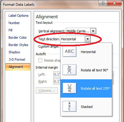
Now choose Alignment in the Format Data Labels Options, then from the drop down list of Text direction choose Rotate all text 270 degree.

There you go. You just added data labels to your chart and the final result is this.

Create a Simple Chart in Excel

---

Today we are going to create a simple Column chart in excel showing sales per year.

Follow these simple steps to create a simple chart in excel. I am using excel 2007 for this example.
Step 1:- Create a simple table in excel as shown in the figure below.

Step 2:- First of all click on an empty cell, then go to Insert > Charts > Column and then click on Stacked Column.

Step 3:- An empty Chart Area will be created. Right click on the Chart Area and then click on Select Data.

Step 4:- Select Data Source dialog box will open. Now click on the Add button as in the image below.

Another pop up dialog box will appear. In the Series name text box select the title sales and in the Series values box click on the first data under sales and then click and drag it up to the last entry of the table.

OR

Click on the first number under Sales hold Shift and then click on the last data.

And then click OK. 

Step 5:- Now the earlier pop up window will reappear but a Series named Sales will appear on the Left hand side. Now click on the Edit button on the right hand side of the window.

One more window will appear. This time select all the years under the title Years and click OK.

Step 6:- Now again click OK on the pop-up window and the final chart will look like this.